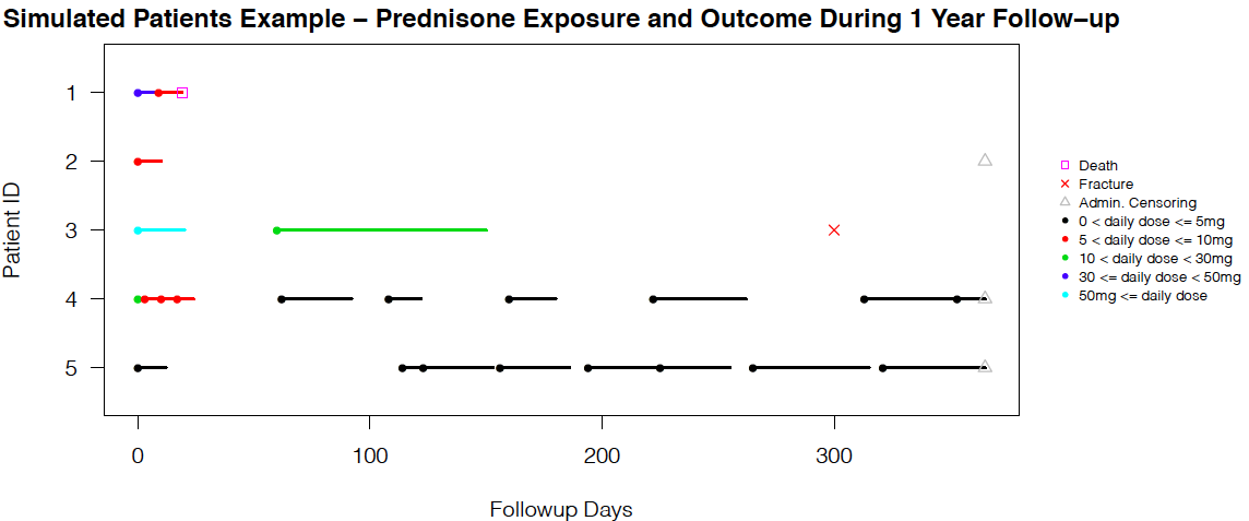
Clinical visits on a discrete-time scale introduce missing data problems, while pharmacy dispensations from administrative data are naturally continuous due to the record linkage feature and can thus avoid such a situation. For many longitudinal pharmacoepidemiological studies, treatment episode construction and dealing with time-varying exposure and confounders are fundamental challenges. We propose the novel method of modeling the dispensation pattern through a stochastic process: marked point process (MPP), and we handle the time-varying confounders through inverse probability treatment weighting.
This repository contains the source code to perform simulation studies with various combinations of the state-of-the-art marginal structural models (MSM) in discrete and continuous-time, and a thorough data cleaning and analysis steps for demonstration. Due to confidentiality reasons, the original data and SAS cleaning code are not presented here, but a full version of the thesis and results are available upon request.
Several R packages need to be installed and loaded for the simulation study. In the data generation and single seed simulation phase, we need library(survival), library(splines), and library(dplyr). Afterwards, we need library(parallel) to perform parallel computing on a Windows system (commented code also available for Mac/OS). Depending on the scenario or time-scale, one simulation study might take up to eleven hours to run, even with parallel setting.
Under Simulation/, we have four independent simulation scenarios, but they share the same structure and naming convention. The directory Simulation/Sim1 contains the files helper_sim1.R, Marginal_sim1.R, and Marginal_sim1_repeat.R for continuous-time exposure models, and helper_sim1_slm.R, Marginal_sim1_slm.R, and Marginal_sim1_repeat_slm.R for discrete models. These set of three files documents the data generating algorithm, the single iteration of simulation, and the repeated 1,000 rounds of simulations running on parallel cores to speed up computing time. Besides, the two .q files are called for case-base sampling robust sandwich variance estimator in both settings [1]. The marginalrate_simple.r documents the numerical integration needed to check the true simulation parameter value [2].
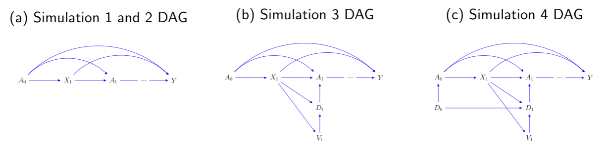
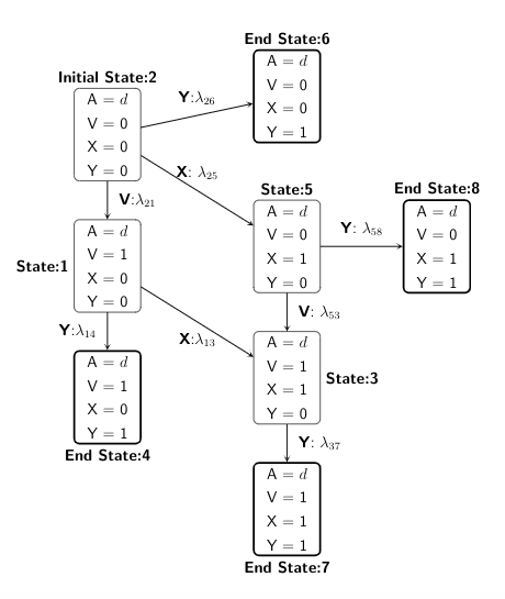
A scenario that patients all start unexposed, and then start the treatment at some individual-specific time point. or
can be interpret as a treatment initiation process, in continuous and discrete time, respectively.
or
is the confounder process, and Y is the time-to-event outcome.
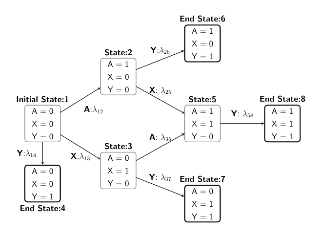
We start with state 1, and then depending on the treatment or confounder or event process taken, the individual can move across different states within administrative censoring of 5 years, with probabilities specified in a transition matrix.
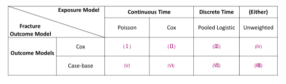
For simualtion 1 and 2, we have the below cross tabulation of exposure weighting and outcome MSM model combinations:
In scenario 2, we simulate a reversed situation of scenario 1. With the new-user cohort design of interest, we have =
= 1 so that everyone starts exposed, and then a change in visit status results in a stop of treatment.
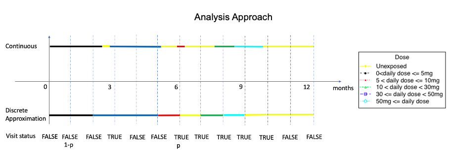
Similar to the second scenario, all patients start with being on treatment, but we separate the modeling of exposure process into a visit process
that induces the corresponding treatment assignment indicator
, where the dosage level is binary, indicating treatment stopping or continuation on the same treatment.
For simualtion 3 and 4, we have the below cross tabulation of model combinations:
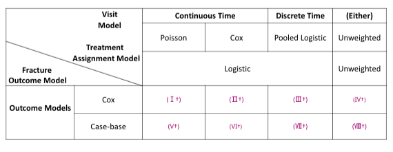
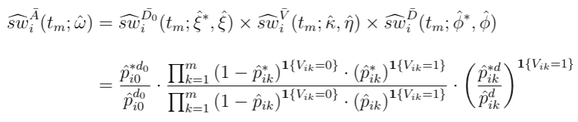
For MPP, the combined weights is the product of stabilized weights from the visiting and dosage models.
Similar to the second and third scenario, all patients start with on treatment, with some initial dose sampled from a logistic model. We also separate the modelling of
into
and
, but we extend the dosage level to three categories, indicating stop treatment, or continue on the same treatment or change to a higher dose treatment. We use a multinomial model for the modeling of
.
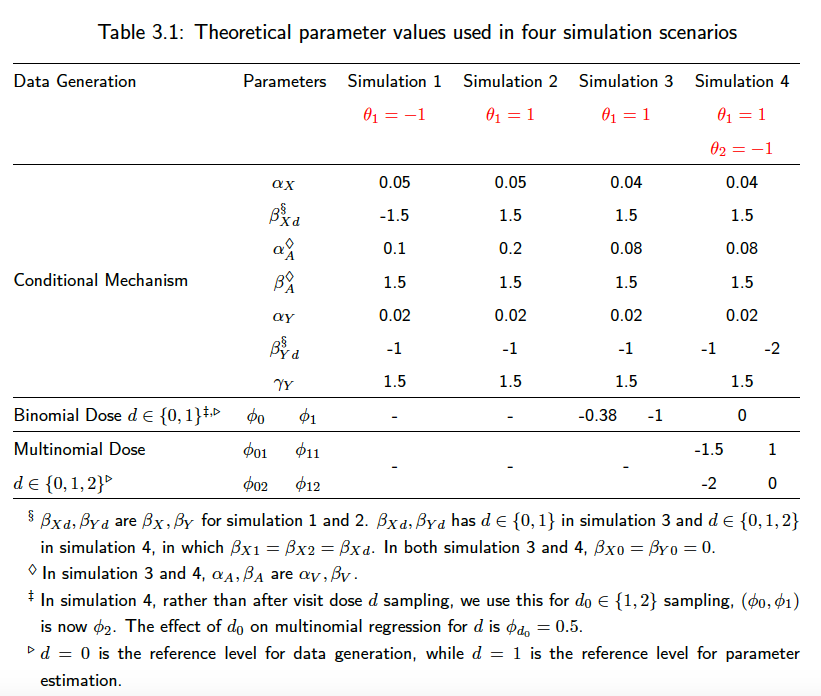
The main simulation parameters can be changed in the helper_.R files under each scenario. We require keeping the discrete and continuous-time parameters the same for the sake of comparison. As a summary of the simulation parameters used in the above four scenarios, we have
Simulation results are presented in tables. The mean, variance, MSE, coverage, and other statistical features are similar across different combinations, but case-base sampling effectively shortened the runtime to 1/5 of that of Cox model.
Required R packages are library(survival), library(plyr), library(dplyr), library(stringr), library(splines), library(survey), library(tableone), library(MASS), library(xtable), library(forestplot), library(Hmisc), library(tidyverse), library(ggplot2), and library(lmtest). A R version of 3.5.2 or above and the packages version as recent as possible are recommended.
Initial data cleaning steps are implemented in SAS (data and code not presented due to confidentiality), but here are some highlights:
- We systematically cleaned the error-prone BP days-supply values based on peer-reviewed guidelines.
- We constructed the non-overlapping treatment and confounder episodes by shifting forward the overlap duration and all subsequent dispensations or truncating the current dispensation duration, depending on whether the overlap is <= 30 days or not.
- We derived fracture outcome by considering a 90 day washout period.
For the purpose of demonstration, under DataAnalysis/Fake_Data_Workflow/, SAS_cleaning_demo.sas is the code used to create and clean the exposure data, and GC_FINAL.csv shows how the exposure dispensation looks like. Then, the other .R files read the GC_FINAL.csv into R and generate the long-format dataset needed for modeling.
The files in DataAnalysis/Real_Data_Final_Workflow/ are the actual R code used for data cleaning, manipulation, visualization, modeling, diagnostic, and potential outcome prediction.
FINAL_Workflow.R is the master file that controls the sourcing of all lower level files. We start with reading in the baseline, exposure, and confounder .csv files by Level4_Clean.R. Several descriptive results can be returned with Table1.R, Dose_line_plot.R, and Death_Fx_Time_plot.R. Then, we generate the five-day interval long-format exposure dataset by Exposure_dataset.R, and fit the exposure models separately for female and male in Exposure_models_female.R or Exposure_models.R. (The commented out files Exposure_models_female_nonum.R or Exposure_models_nonum.R only differ by removing baseline covariates from the marginal model (numerator of stabilized weights), and we use these two files to get the exposure models needed for standardized mean difference (SMD) diagnostics plots [3] at baseline only.)
Afterwards, we can save the exposure model outputs as tables and forest plots by running the automated files on Model_Outputs_names.R and Model_Outputs.R. We then generate the case-base sampled long-format outcome dataset by Outcome_dataset.R. After the exposure weights are predicted and mapped over to the outcome dataset, we can perform the diagnostics via generating the stabilized weights distribution and as a function over time plots in Diagnostics.R. Then, the time-dependent SMD plots over three time points can be plotted with DiagnosticSMD.R.
We can then fit the outcome models by Outcome_models.R, and return the outcome model output tables by running Model_Outputs.R again. Then the descriptive hazard plot and potential hazard data set construction and plots are returned by Hazard_over_time_plt.R.
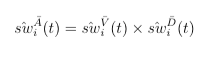
The combined weighting function is the cumulative product of stabilized (marginal divided by conditional) weights from the intial dose assignment, the subsequent visiting, and the subsequent dose assignment model. Depending on if an individual is getting a new dispensation during follow-up, the visiting and dosage weights can be muted, but the baseline weights always exist.
After using weighting to remove time-dependent confounders, several baseline characteristics are predictive for fracture. In terms of potential hazard under always treated with each dose level, 30-50mg daily has the highest impact on fracture. The impact of GC on fracture has the steepest escalation during the first 30 days and starts to reach a plateau after 3 months, with a slight increase near the end of the one year follow-up.
[1]: Lumley, T. and Heagerty, P. (1999). "Weighted empirical adaptive variance estimators for correlated data regression." Journal of the Royal Statistical Society: Series B (Statistical Methodology), 61(2):459-477. [https://www.jstor.org/stable/2680652?seq=1]
[2] Saarela, O. and Liu, Z. (2016). "A flexible parametric approach for estimating continuous-time inverse probability of treatment and censoring weights". Statistics in medicine, 35(23):4238-4251. [https://onlinelibrary.wiley.com/doi/10.1002/sim.6979]
[3] Tang, T.-S., Austin, P. C., Lawson, K. A., Finelli, A., and Saarela, O. (2020). "Constructing inverse probability weights for institutional comparisons in healthcare." Statistics in Medicine. [https://onlinelibrary.wiley.com/doi/abs/10.1002/sim.8657]
MIT License
Copyright (c) 2021 Estella Yixing Dong
Permission is hereby granted, free of charge, to any person obtaining a copy of this software and associated documentation files (the "Software"), to deal in the Software without restriction, including without limitation the rights to use, copy, modify, merge, publish, distribute, sublicense, and/or sell copies of the Software, and to permit persons to whom the Software is furnished to do so, subject to the following conditions:
The above copyright notice and this permission notice shall be included in all copies or substantial portions of the Software.
THE SOFTWARE IS PROVIDED "AS IS", WITHOUT WARRANTY OF ANY KIND, EXPRESS OR IMPLIED, INCLUDING BUT NOT LIMITED TO THE WARRANTIES OF MERCHANTABILITY, FITNESS FOR A PARTICULAR PURPOSE AND NONINFRINGEMENT. IN NO EVENT SHALL THE AUTHORS OR COPYRIGHT HOLDERS BE LIABLE FOR ANY CLAIM, DAMAGES OR OTHER LIABILITY, WHETHER IN AN ACTION OF CONTRACT, TORT OR OTHERWISE, ARISING FROM, OUT OF OR IN CONNECTION WITH THE SOFTWARE OR THE USE OR OTHER DEALINGS IN THE SOFTWARE.