4a. Interpreting the Results of DRAM
So you have successfully ran DRAM or DRAM-v through the annotate and distill steps. Now you want to know what each of the MAGs or metagenomes are capable of. The recommended workflow for running DRAM and DRAM-v is to always annotate and then distill. By starting with the product, the most distilled part of the pipeline, then looking to the distillate and then raw data will make analyzing genomes the most helpful.
Start by getting your product.html file to a local environment (e.g. download the file if it is on a server) then open it in an internet browser window. This file is totally independent and can be shared without needing to share any other data. When you open that window you will get something that will look like this. It is a heatmap where the y-axis represents the different genomes that have been analyzed and the x-axis represents various functions genomes can be capable of. This gives out an overview of the major metabolic functions that each genome you have annotated is capable of.
In addition to the product html file a table containing the same information is also generated called product.tsv.
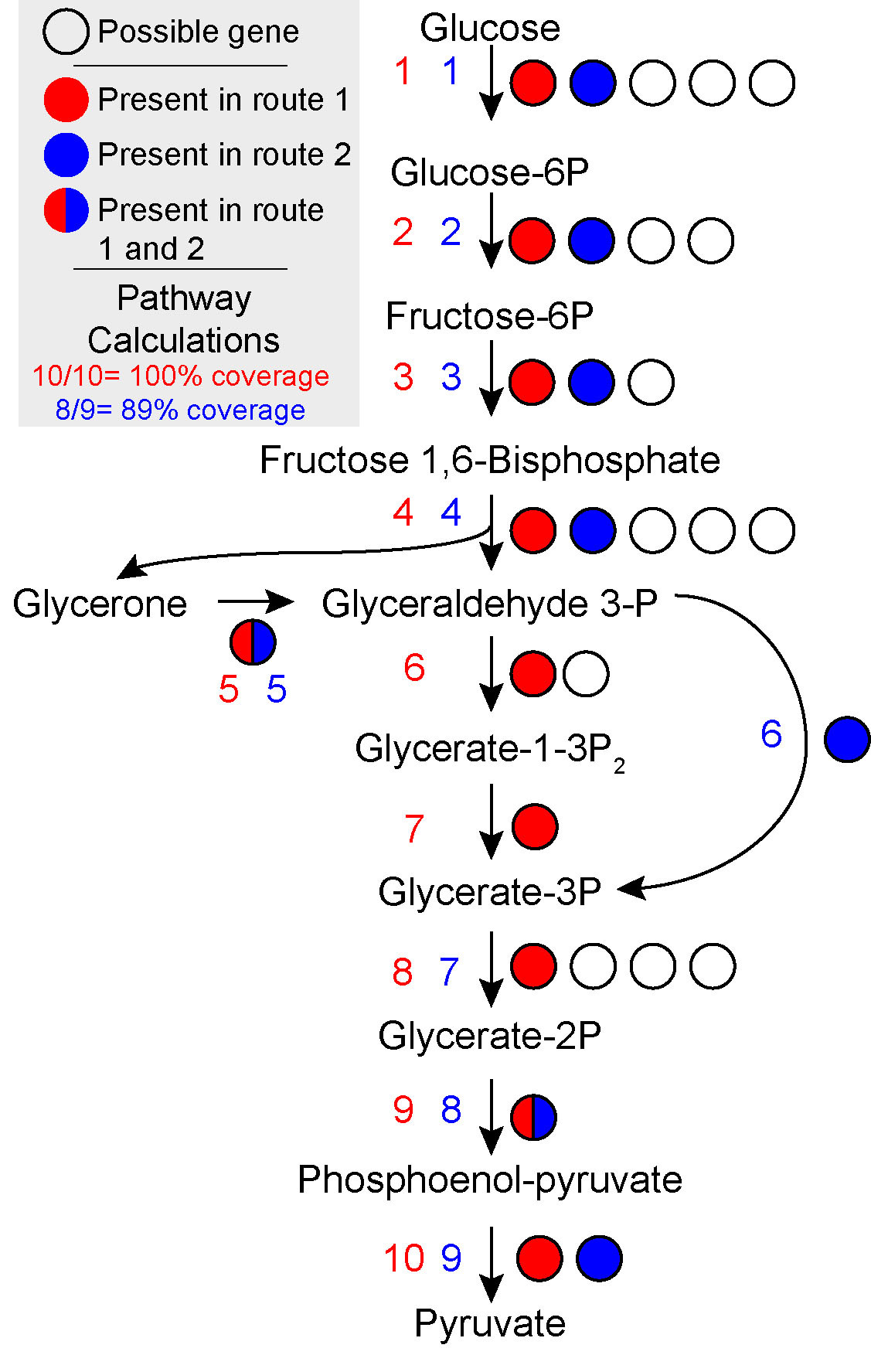
The farthest left section of the heatmap is labelled module and gives the completion of various pathways representing common, relevant metabolisms. The color of each cell of the heatmap represents the completeness of that module. DRAM measures completeness by looking at the individual steps of a module and checking if at least one gene is present in each step. Therefore all genes in a module or even all subunits of all genes of one path through a module need to be present in order for the coverage of a module to be presented as 100% covered (see figure below). To see more detail about the coverage of a module you can jump to using the distillate.
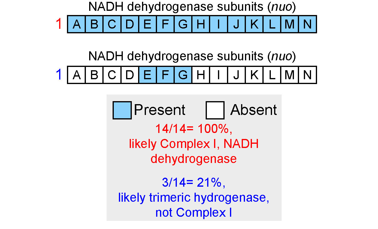
The next section of the product shows the presence of various electron transport chain complexes. This allows the user to rapidly understand the ability of microbes to perform aerobic respiration. Like with modules the color of the individual cells of the heatmap shows the coverage of that electron transport chain complex. Coverage is calculated differently from modules though. Here the complete path through a module is considered and to be fully covered a complete set of annotations from any valid path through the module must be present (see figure below).
The remainder of the heatmap is based on checking whether or not certain annotations are present which are indicative of characteristic metabolic functions being present. Each cell is shaded based on the presence or absence of the function for that column. Each cell is represented by a list of annotation ID's that can come from any of the databases that DRAM annotates against. If any one of the annotation ID's from that list is present in a genome then the cell is lit up to represent a true finding. For some functions the presence of just one gene is not enough to say that function is present. For these functions there are multiple columns with the same name but multiple parts (e.g. Xyloglucan, pt. 1; Xyloglucan, pt. 2; and Xyloglucan, pt. 3). For these functions all parts must be lit up as being present to consider the genome to encode that function. It is critical to remember that absence of evidence is not evidence of absence. If a function is absent that may be because that gene was not part of the assembly of the genome or it is a gene that is difficult to annotate accurately. Finding and annotating this gene in a more detail manual way may be something you want to pursue if you are particularly interested in a certain function.
The distillate comes in the form of two files which contain detailed information about the metabolic functions annotated in each genome and information about the quality and taxonomy of each genome.
Where the product gives a brief overview of the metabolic functions that each genome is capable of the metabolism summary gives an accounting of the abundance of a wide variety of genes including those representing common metabolisms. The functions are a part of a hierarchy. The highest level is the sheet which represents broad functions (e.g. carbon utilization) or cellular functions (e.g. transporters). These represent very broad categories. The next category is the header and the (optional) subheader. Below this is the module. The modules in the distillate include KEGG modules, CAZy genes separated by substrate, MEROPs genes, tRNAs and other custom modules.
This table comes in the form of a excel formatted spreadsheet with multiple sheets representing the highest level of the hierarchy. The first five columns give information about the annotation and the remaining columns give the count of genes with that annotation in each of the genomes analyzed. The gene_id and gene_description columns give the finest level of detail about the function present. The next column is the module that this gene is a part of, followed by the header and optional subheader.
The file genome_stats.tsv gives the required information for the MIMAG requirements so that users can evaluate the quality of their genomes. To add taxonomy, completeness and contamination the user must provide results files from GTDBTk and checkM checkM. Additionally the number of scaffolds in the genome is provided along with the rRNA locations as determined by barrnap and the number of tRNAs present (if tRNAscan-SE was ran).
In the raw annotations are the types of files returned by most genome annotators. This ranges from scaffold and genome feature files to tables with all the recorded annotations. These are the files you will want to dig into if your metabolism or gene function of interest is not covered by the distillate and product or you need more detail than these levels of summarization provide.
The file annotations.tsv contains all annotations for all predicted open reading frames. Each row is an individual gene and all columns give annotation information. The first column gives the assigned gene name and subsequent columns give the name of the FASTA file and name of the scaffold that the gene was called from. Next is the gene position on the scaffold (1-end), the nucleotide start position, nucleotide end position and the strandedness of the gene. After that is the rank of the annotation. The rank is assigned by Ranks are assigned based on the methods outlined in Daly, et al. 2016. Briefly an annotation is given an A rank if there is a reciprocal best hit to a KEGG gene, a B if there is a reciprocal best hit to a UniRef90 gene, a C if there is a forward hit only to either KEGG or UniRef90, a D if there is only a hit to PFAM and an E if there is no annotation to KEGG, UniRef90 or PFAM.
The subsequent columns give the annotation information. For databases with BLAST-style (done using MMseqs2) searches columns with the database hit ({database}_hit), if the hit was a reciprocal best hit ({database}_RBH), the percent identity of the match ({database}_identity), the bitscore of the hit ({database}_bitScore) and the E-value of the hit ({database}_eVal). If the database has specific identifiers that DRAM pulls then an additional column is present ({database}_id). These are the identifiers that are used in the distillation of annotations.
For databases that are searched using HMMs (using HMMER) only a list of hits is given. The hits are separated by semicolons and after each hit in square brackets is the identifier that is associated with the hit. The identifier is what is used in the distillation of the annotations.
After that is the MHC count (heme_regulatory_motif_count). This is a count of the number of times the CXXCH is present in that gene. Iron-reducing microorganisms use multi-heme c-type cytochromes (MHCs) as terminal reductases for the final step of electron transfer. We note, this is the first step in identifying MHCs, thus to further validate MHC potential, users should look at the annotation (e.g. nitrate reductases should not be considered MHCs), upload into psortB to obtain location information, and perform sequence similarity network analysis relative to known MHCs.
If the GTDBTk results file is given then a column with the taxonomy will be added (bin_taxonomy) and if the checkM is provided then columns will be added with the completion and contamination of the bin the gene is from.
Three FASTA files are generated by DRAM: scaffolds.fna, genes.fna and genes.faa. The scaffolds file has all scaffolds from all input MAGs with the renamed format to match the annotations table and output gff file. genes.fna has all genes from all MAGs as nucleotides and genes.faa has all genes from all MAGs as amino acids.
Annotations are given in two formats that can be used for subsequent analysis or visualization. These file contain all open reading frames with annotations as well as tRNAs and rRNAs. The genes.gff file contains all genes from all MAGs and matches with the scaffolds.fna file. There is a directory called genbank which has one genbank file per genome. These can be used to visualize genomes using any genome viewer.
tRNAs are summarized in tRNAs.tsv and rRNAs are summarized in rRNAs.tsv.
Once you have explored the annotations of your genomes or metagenomes you may want to continue your analysis with other tools. DRAM outputs formats that are compatible with other tools as well as provides DRAM strainer to pull the sequences of interesting genes based on annotations or other characteristics.
If you want to measure differential abundance or expression of genes you can use the outputs of DRAM to get this process started. By mapping your reads to the scaffolds.fna file produced by DRAM you can have mapping to all of your genomes. Additionally if you would like to use tools CuffLinks or StringTie to assemble transcripts and quantify their abundance you can use the genes.gff file from DRAM along with scaffolds.fna, the results of which can be used for differential expression. This will make it so that you can quickly find interesting candidate genes and then you can connect these to the full annotations.tsv in order to learn about their function.
Additionally if you want a quicker analysis you can map directly to the predicted gene sequences in the genes.fna file using a tool like BBmap and again use the full annotations to better understand your abundant or differentially abundant genes.
You might find by looking at your product or genome summary file that there is a metabolism that is common in your community or you may have a metabolism of interest that you would like to more deeply interrogate. A common task here is to identify genes of interest and make a tree in order to understand the relationship between these genes.
For example you might have noticed that pmoA or amoA seem to be common in some of your genomes. To tell these genes apart a tree must be made. Both pmoA and amoA genes are given the KEGG identifier K10944. To do this you can use DRAM strainer to pull all your genes with the KEGG ID using this command: DRAM.py strainer --identifiers K10944 -i annotations.tsv -f genes.faa -o amoa_pmoa_genes.faa. This will give you a FASTA file that you can use as input to multiple sequence alignment and tree making software so that you can understand whether these genes are acting on methane or ammonia.
Many proteins with catalytic function are embedded into cell membranes. While DRAM cannot directly identify if a protein seems to be membrane bound other tools such as psortB can be used for this function. Glycoside hydrolases are often membrane bound and the product in a DRAM analysis may have shown that chitin utilization via GH18 is common in your set of genomes. You can use DRAM strainer to get this genes using this command: DRAM.py strainer --identifiers GH18 -i annotations.tsv -f genes.faa -o GH18_genes.faa. The genes in that file can then be used as input to psortB to learn about their membrane bound nature.