This project aims to visualize filters, feature maps, guided backpropagation from any convolutional layers of all pre-trained models on ImageNet available in tf.keras.applications (TF 2.3). This will help you observe how filters and feature maps change through each convolution layer from input to output.
With any image uploaded, you can also make the classification with any of the above models and generate GradCAM, Guided-GradCAM to see the important features based on which the model makes its decision.
If "art" is in your blood, you can use any model to generate hallucination-like visuals from your original images. For this feature, personally, I highly recommend trying with "InceptionV3" model as the deep-dream images generated from this model are appealing.
With the current version, there are 26 pre-trained models.
- Clone this repo:
git clone https://github.com/nguyenhoa93/cnn-visualization-keras-tf2
cd cnn-visualization-keras-tf2- Create virtualev:
conda create -n cnn-vis python=3.6
conda activate cnn-vs
bash requirements.txt- Run demo with the file
visualization.ipynb
- Go to this link: https://colab.research.google.com/github/nguyenhoa93/cnn-visualization-keras-tf2/blob/master/visualization.ipynb
- Change your runtime type to
Python3 - Choose GPU as your hardware accelerator.
- Run the code.
Voila! You got it.
| Method | Brief |
|---|---|
| Filter visualization | Simply plot the learned filters. * Step 1: Find a convolutional layer. * Step 2: Get weights at a convolution layer, they are filters at this layer. * Step 3: Plot filter with the values from step 2. This method does not require an input image. VGG-16, block1_conv1 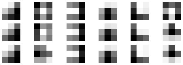 |
| Feature map visualization | Plot the feature maps obtained when fitting an image to the network. * Step 1: Find a convolutional layer. * Step 2: Build a feature model from the input up to that convolutional layer. * Step 3: Fit the image to the feature model to get feature maps. * Step 4: Plot the feature map. VGG-16, block1_conv1 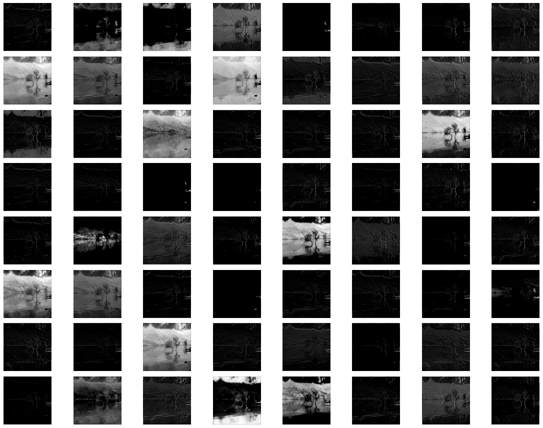 VGG-16, block5_conv3 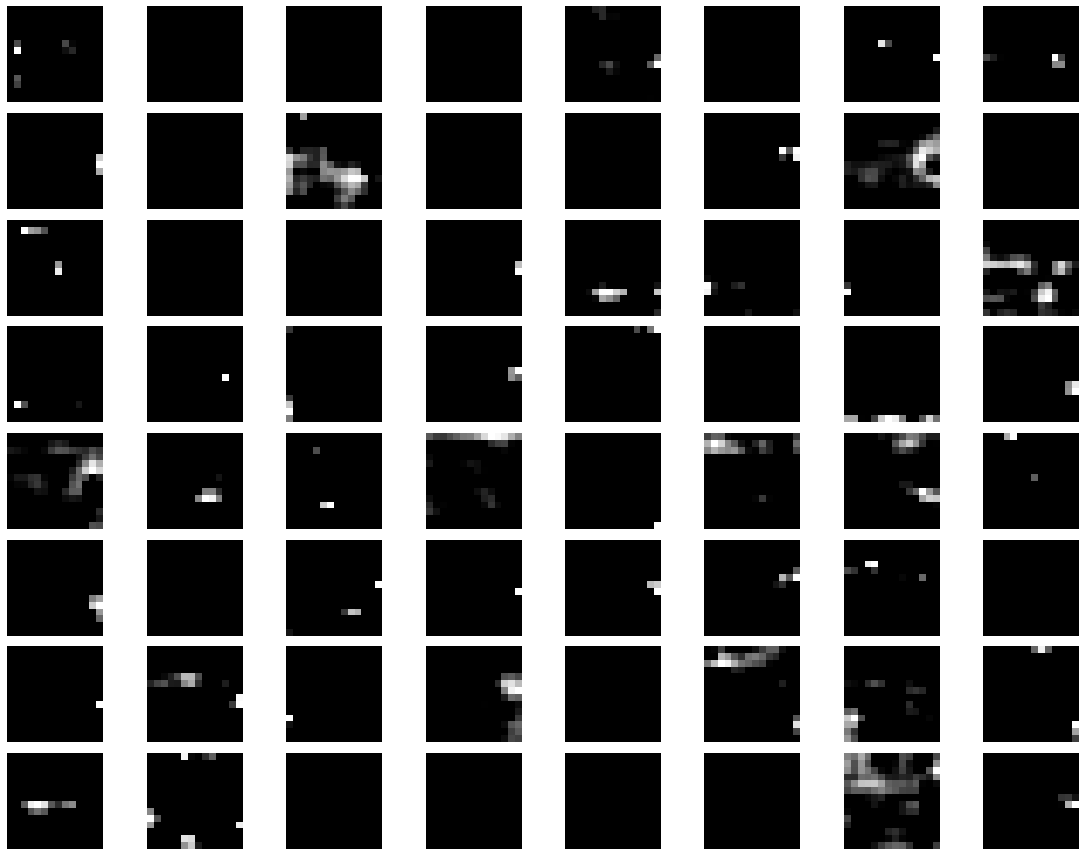 |
| Guided Backpropagation | Backpropagate from a particular convolution layer to input image with modificaton of the gradient of ReLU. VGG-16: block1_conv1 & block5_conv3 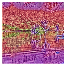 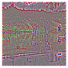 |
| GradCAM | * Step 1: Determine the last convolutional layer * Step 2: Perform gradient from `pre-softmax` layer to last convolutional layer and the apply global average pooling to obtain weights for neurons' importance. * Step 3: Linearly combinate feature map of last convolutional layer and weights, then apply ReLu on that linear combination. InceptionV3, explanation for "lakeside" class 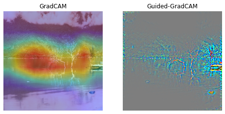 |
| Guided-GradCAM | * Step 1: Calculate guided backpropagation from last convolutional layer to input. * Step 2: Upsample GradCAM to the size of input * Step 3: Apply element-wise multiplication of guided backpropagation and GradCAM InceptionV3, explanation for "boathouse" class 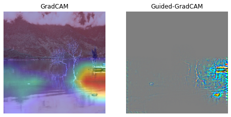 |
| Deep Dream | See more in this excellent tutorial from François Chollet: https://keras.io/examples/generative/deep_dream/ InceptionV3 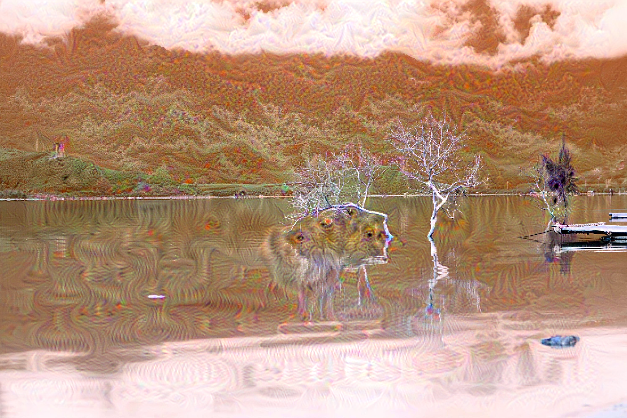 |
Original image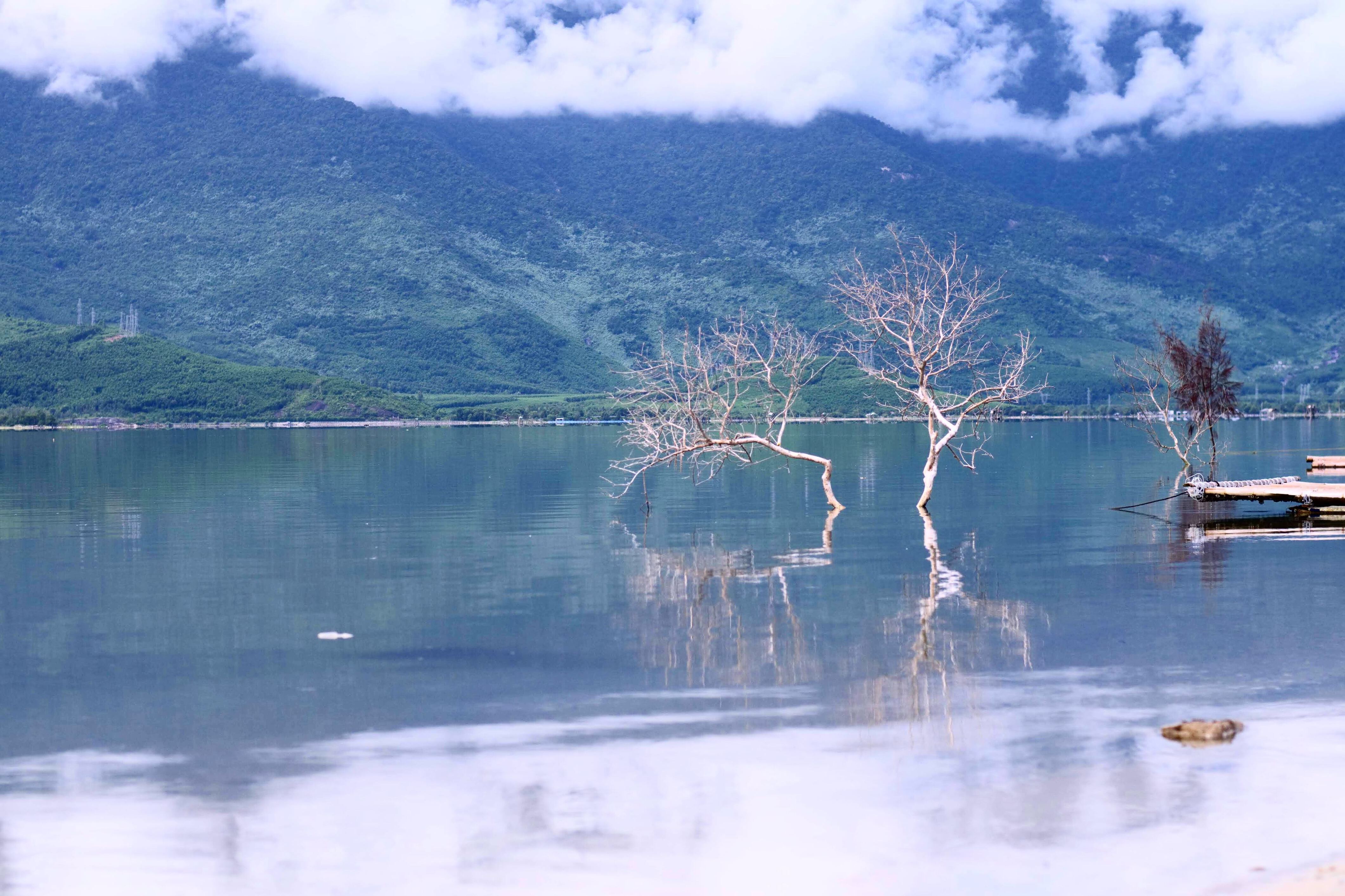 | |
- How to Visualize Filters and Feature Maps in Convolutional Neural Networks by Machine Learning Mastery
- Pytorch CNN visualzaton by utkuozbulak: https://github.com/utkuozbulak
- CNN visualization with TF 1.3 by conan7882: https://github.com/conan7882/CNN-Visualization
- Deep Dream Tutorial from François Chollet: https://keras.io/examples/generative/deep_dream/
